Welcome to this tutorial covering OpenCV. This type of program is most commonly used for video and image analysis such as license plate reading, facial recognition, robotics, photo editing and more within C++, Python, C and Java. In this tutorial we’ll cover OpenCV for image analysis.
Firstly, the “CV” part in OpenCV as mentioned in the title stands for “Computer Vision” and Image Processing is just a small part of Computer Vision. Let’s take a few steps back. What is Computer Vision?
 As the definition on techopedia:
 According to OpenCV homepage, OpenCV is:
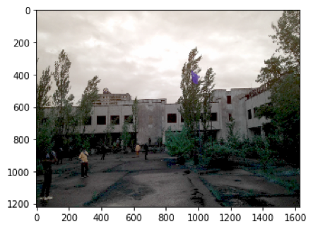
 This image is named “gentleman.jpg”, use the below code to extract the histogram.
 s = T(r)
 We will use gamma correction method to make it have a better brightness:
 Take note of the difference. It’s like magic, right? The result:
 As you can see, the background really has no white in it at all. Everything is dim, but also everything is varying. On the left side, we have enough light to read the text, while the rest of the image is quite dark and requires a bit of focus to even try to read the text.
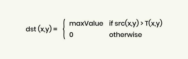
So, in order to apply the threshold, we use THRESH_BINARY threshold type. The function transforms a grayscale image to a binary image according to the formula below:
As you can see, the background really has no white in it at all. Everything is dim, but also everything is varying. On the left side, we have enough light to read the text, while the rest of the image is quite dark and requires a bit of focus to even try to read the text.
So, in order to apply the threshold, we use THRESH_BINARY threshold type. The function transforms a grayscale image to a binary image according to the formula below:
 For the method ADAPTIVE_THRESH_GAUSSIAN_C , the threshold value T(x, y) is a weighted sum (cross-correlation with a Gaussian window) of the blockSize x blockSize neighborhood of (x, y) minus C . The default sigma (standard deviation) is used for the specified blockSize. So we have the code:
 We have just briefly covered the topic of Computer Vision and how to use the OpenCV Library for Python to demonstrate several very basic levels of image processing. We hope that you will have a point of view of computer vision in general and image processing in particular. Yes, it is very basic but as you can see, it is very powerful.
All source code and the result as demonstrated above were documented in a Jupyter notebook which you can download here.
We have just briefly covered the topic of Computer Vision and how to use the OpenCV Library for Python to demonstrate several very basic levels of image processing. We hope that you will have a point of view of computer vision in general and image processing in particular. Yes, it is very basic but as you can see, it is very powerful.
All source code and the result as demonstrated above were documented in a Jupyter notebook which you can download here.
As the definition on techopedia:
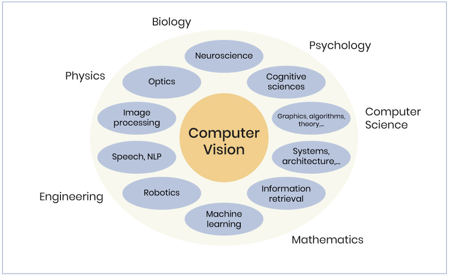
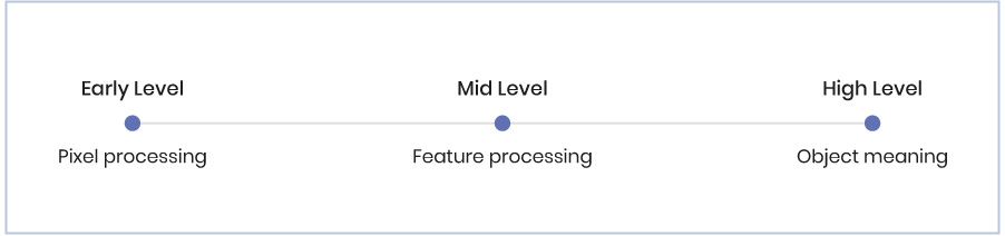
Computer vision is a field of computer science that works on enabling computers to see, identify and process images in the same way that human vision does, and then provide appropriate output. It is like imparting human intelligence and instincts to a computer. In reality though, it is a difficult task to enable computers to recognize images of different objects.Computer vision is closely linked with artificial intelligence, as the computer must interpret what it sees, and then perform appropriate analysis or act accordingly. Nowadays, a huge amount of computer data is generated day in and day out and with the growth and expansion of technology, computers today have the ability to depict vision and process images far more better than the human eye. In Computer Vision, there are 3 levels of processing images which are divided into 3 levels:
According to OpenCV homepage, OpenCV is:
OpenCV (Open Source Computer Vision Library) is released under a BSD license and hence it’s free for both academic and commercial use. It has C++, Python and Java interfaces and supports Windows, Linux, Mac OS, iOS and Android. OpenCV was designed for computational efficiency and with a strong focus on real-time applications. Written in optimized C/C++, the library can take advantage of multi-core processing. Enabled with OpenCL, it can take advantage of the hardware acceleration of the underlying heterogeneous compute platform.So, in order to start with Computer Vision or Image Processing in particular, it is recommended to first start with OpenCV. Are you ready to begin? For installation and settings, you can refer to this article on MacOS. Basically, you’ll need Python, OpenCV library for Python, numpy and matplotlib.
1. Basic definitions and theories
Image representation
Image representation is an image of dimensions. M×N is defined by the function b with: b: DM x DN → In Where DM = {1, 2, …, M}, DN = {1, 2, …, N} and n = 1, 2, 3,…Pixel
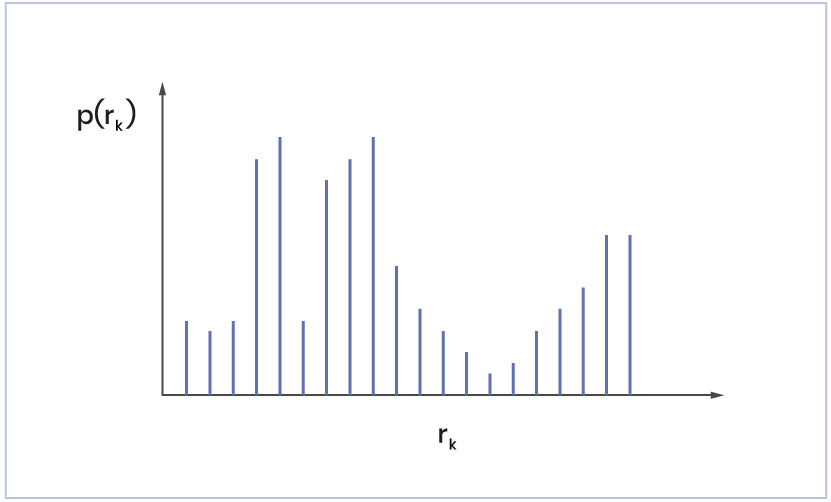
The smallest part of an image is the pixel so we can call it a picture element. It is characterized by its position (i, j) and the intensity vector b(i, j).Image histogram
If we represent an image in black-and-white color, each pixel in the image has a value that represents the amount of light. It only stands for intensity information. So, if we have a digital image with a gray level in the range of [0, L-1]. A histogram is a plot that shows the “probability” p(rk) of the occurrence of gray- level rk with: p(rk) = nk/N- rk is the kth gray level
- nk is number of pixels with kth gray level
- N is total number of pixels
- k = 0, 1, 2, 3, 4, 5, …, L-1
Example of a histogram
Histograms reveal a lot about an image. We will dive deeper into that later.1. Applications
First steps
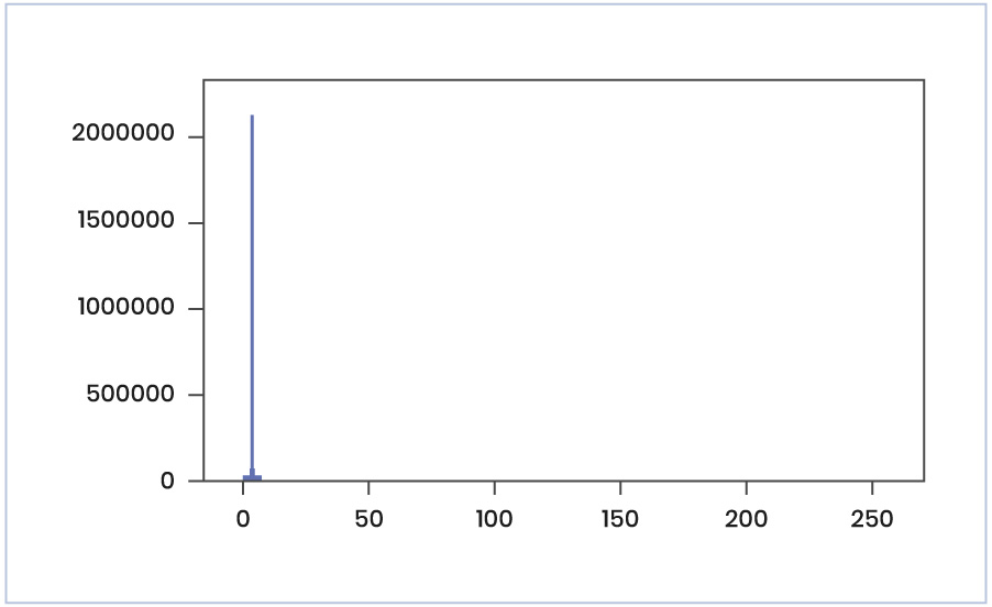
We will verify if you are ready to work with OpenCV. First, create a .py file and import the necessary libraries like below:import cv2 import matplotlib import numpyIf you don’t have any problems running this file then you are ready to continue. Now, to have a very first application of OpenCV, we will first start with the histogram of an image below.
This image is named “gentleman.jpg”, use the below code to extract the histogram.
import cv2
import numpy as np
from matplotlib import pyplot as plt
img = cv2.imread('gentleman.jpg',0)
plt.hist(img.ravel(),256,[0,256])
plt.show()
The image has a lot of dark-color parts. This is reflected in the chart as you can see the number of pixels with low level of light is very high. The result:
Gamma correction
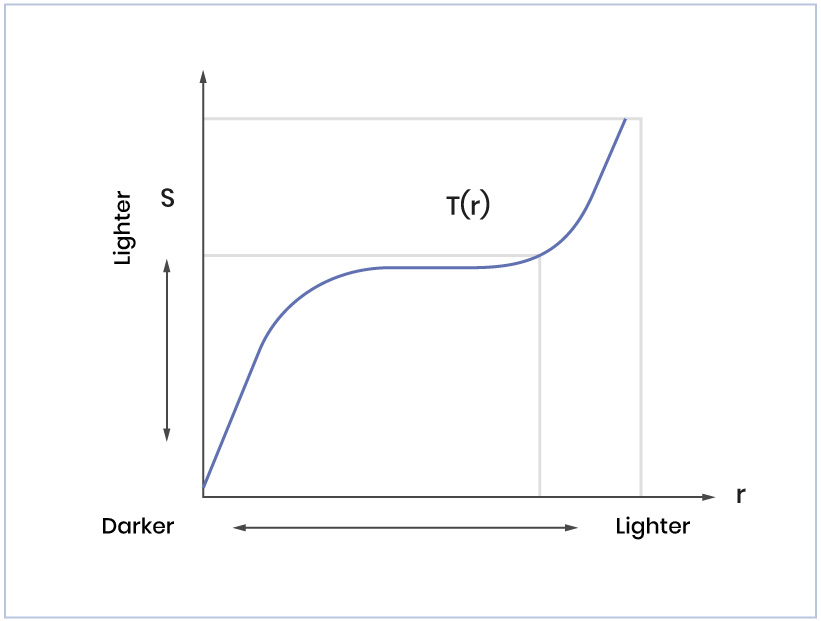
Correction (Enhancement) is to make an image more suitable than the original one for a specific application. Gamma correction method is useful when you want to change the contrast and brightness of an image. To understand about gamma correction, first we need to understand about Power Law Transformation. With input images f(x, y), and after transformation T, we have the enhanced output image g(x, y): g(x, y) = T[ f(x, y) ] If we denote r, s as the gray level of f(x, y) and g(x, y) for any point (x, y), the formula can be written as:
s = T(r)
An example of T
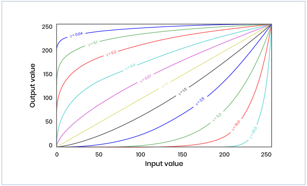
In the above example, for any gray level value, in the x-axis, we have the corresponding value in the y-axis as the result of the transformation. So, to enhance the brightness of the image, we will change the value r to reach the value s. The Power Law Transformation is defined to do the work, and its form is: s = c*ry The above transformation uses r power γ (gamma), so it is called Power Law Transformation. By changing the value of γ, we have different results. So the gamma correction is the process of choosing the best value for gamma to have the best output image.
Plot for different values of gamma
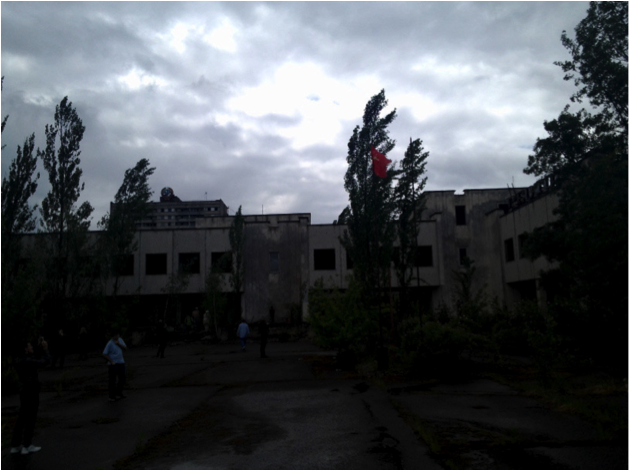
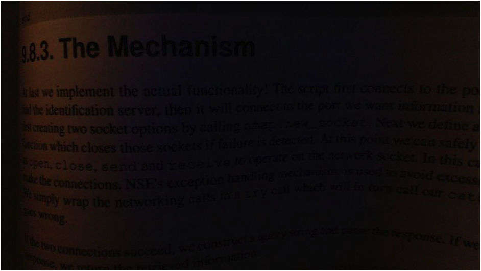
When γ < 1, the original dark regions will be brighter and the histogram will be shifted to the right whereas it will be the opposite with γ > 1. For this demonstration, we will use a really dark photo like the one below:
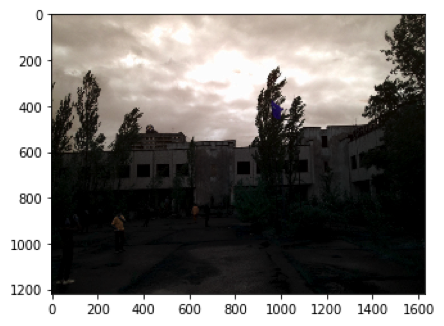
We will use gamma correction method to make it have a better brightness:
import cv2
import numpy as np
from matplotlib import pyplot as plt
darkImage = cv2.imread('dark.png')
plt.imshow(darkImage)
plt.show()
def adjust_gamma(image, gamma=1.0):
   table = np.array([((i / 255.0) ** gamma) * 255
                     for i in np.arange(0, 256)]).astype("uint8")
   # apply gamma correction using the lookup table
   return cv2.LUT(image, table)
plt.imshow(adjusted)
plt.show()
Take note of the difference. It’s like magic, right? The result:
Thresholding
The idea behind thresholding is really simple. At the most basic level, thresholding is used to convert everything to white or black, based on a threshold value. By making use of the gray level, if the threshold is 125 (out of 255), then any value that was 125 and under would be converted to 0 (it means black), and everything above 125 would be converted to 255 (it means white). Normally, we will convert the input image to gray-scale before applying threshold. In order to demonstrate this method, let’s look at a really dark book page like the one below:
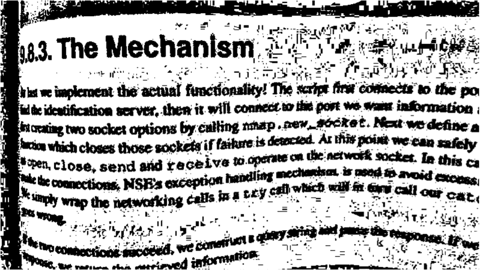
As you can see, the background really has no white in it at all. Everything is dim, but also everything is varying. On the left side, we have enough light to read the text, while the rest of the image is quite dark and requires a bit of focus to even try to read the text.
So, in order to apply the threshold, we use THRESH_BINARY threshold type. The function transforms a grayscale image to a binary image according to the formula below:
For the method ADAPTIVE_THRESH_GAUSSIAN_C , the threshold value T(x, y) is a weighted sum (cross-correlation with a Gaussian window) of the blockSize x blockSize neighborhood of (x, y) minus C . The default sigma (standard deviation) is used for the specified blockSize. So we have the code:
import cv2
import numpy as np
from matplotlib import pyplot as plt
img = cv2.imread('bookpage.jpg')
plt.imshow(img)
plt.show()
grayscaled = cv2.cvtColor(img,cv2.COLOR_BGR2GRAY)
th = cv2.adaptiveThreshold(grayscaled, 255, cv2.ADAPTIVE_THRESH_GAUSSIAN_C, cv2.THRESH_BINARY, 115, 1)
plt.imshow(th)
plt.show()
cv2.waitKey(0)
cv2.destroyAllWindows()
Now, we have the output version of the book page in black and white which makes the page much easier to read.
We have just briefly covered the topic of Computer Vision and how to use the OpenCV Library for Python to demonstrate several very basic levels of image processing. We hope that you will have a point of view of computer vision in general and image processing in particular. Yes, it is very basic but as you can see, it is very powerful.
All source code and the result as demonstrated above were documented in a Jupyter notebook which you can download here.